Sorting
| Algorithm | complexity | extra space | stable |
|---|---|---|---|
| selectionsort | N^2 | 1 | N |
| insertionsort | N to N^2 *NlogN to (NlogN)^2 |
1 | Y |
| shellsort | NlogN (still unknown) | 1 | N |
| quicksort | NlogN *N(logN)^2 |
1gN | N |
| 3-way quicksort | NlogN *N to NlogN |
1gN | N |
| R-way quicksort | NlogN/logR *N to NlogN/logR |
N + bucket size? | N |
| mergesort | NlogN *N(logN)^2 |
N | Y |
| heapsort | NlogN | 1 | N |
| Key-indexed counting | *(11N + 4R) | N | Y |
| LSD | *(NW) | N | Y |
| MSD | *N to Nw (NlogN/logR on average) | N + WR | Y |
| 3-way string quicksort | *N to Nw (2NlnN on average) | W + logN | N |
In the above table, we listed the order of growth to sort N items. By default, the cost is count by number of items. The items can be numbers, Strings, Comparable objects. When the items are Strings, we mark the cost with *, for string item, the cost is measured as number of calls to charAt() to sort N strings from a R-character alphabet. The average string length is w, the max string length is W. Some algorithms only applied to string items, for example key-indexed counting, LSD, MSD and 3-way string quicksort.
As we saw from the above comparison. Selection sort have O(N^2) computation complexity, therefore not practical for large sorting work. They only need O(1) space and incrementally produce results, which makes them still good choices on simple resource limited devices. Insertion sort is fast on almost sorted collection and is stable. shellsort, quicksort, mergesort and heapsort have the same O(NlogN) performance. The in place swapping sorting algorithm shellsort and heapsort has the advantage on resource limited environment. These 2 sorting algorithm are not stable, they sometimes move elements back and forth. Putting O(lgN) space resource, quicksort performs better than shellsort and heapsort on randomly shuffled collections. It is however still unstable. Putting more space resource O(N), the mergesort stably achieve O(NlogN) performance. The radixsort's performance can get close to O(N) when the max length of the sorting number is small compare to the to the total number to sort. It needs space resource O(N) and is stable too. The space is extra space needed during the sort, we always need N space for storing the array elements.
Soft Math:
When divide and conquer approach is used, the cost is proportional to N multiply a Logarithm function of N. The intuition is:
Each of the N items has N possible positions to take. Each one of the N items needs to make a number of decisions to find its final position among N possibilities. The ordered array has nothing special, it is just one of the possible result of these decision makings.
For each decision, if we have R choices, the number of possibilities fan out at each decision. Imagine we are making a decision tree. In order to create N possibilities, n decisions need to be make. R^n = N, where n is the Logarithm function of N with R as the base. The N node decision tree can be tall or short, depending on both N and R. More choices suggest more space needed, but shorter trees means faster approaching goal.
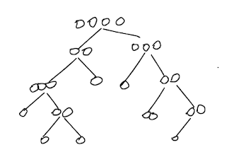
Binary decision tree, for example, has 2 choices at each decision. The n decisions create 2^n = N possible positions after n dividing. In another word, a n depth binary search tree has N nodes. Let's imagine the N items are individuals choose a seat on a binary search tree. For each one of the N items, the individual item has to make on average n decisions to sink to its final position. It took roughly Nn total decision makings for the group to have all N items positioned on a binary decision tree. A binary decision tree is already ordered (top-down merge sort). So the total cost is proportional to Nn = NlgN.
 |
| binary decision tree with n = 4 and N = 16 |
Quick sort, also put N items on a binary decision tree, roughly speaking. At each step, we make a decision to move the element left or right, or, stay un-move. The stay is also a decision. So the R is a little bit bigger than 2. No wonder quick sort, which put N items on 1 + 2 + 4 + ... + 2^n = N possible positions on a binary search tree, is faster than merge sort (R=2) for random numbers.
 |
| binary search tree with n = 4 and N = 29 |
Let's don't ignore the word random. For merge sort, half of the items make left decision, half of the items make right decision. The tree is a symmetric one. Quick sort decision tree, on the other hand, is a random one. The items move to the left of the pivotal or right of the pivotal most likely are not half and half. We have to have N random items to make lots of random decisions to make the decision tree looks like a healthy balanced binary search tree. A healthy binary search tree makes quick approach, an unbalanced binary search tree, ugly standing up there, makes pool performance. With statistics for randomness, the cost expression is usually based with e, proportional to NlnN.
3-way quick sort, makes 3 decisions, left, right, middle, with middle portion bigger than that of the quick sort, the performance is even better. More equal components there are, better performance the 3 way quick sort has.
 |
| binary search tree with equal node elements |
We can predict R-way quick sort will perform even better than 3-way quick sort with larger memory cost.
 |
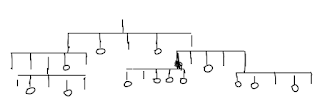
| R-way decision tree with bucket size R = 5 |
With the above main frame of N individuals choosing paths on a N-state decision tree, we now add an important detail -- when an individual makes a decision, that decision is not random, it involves comparison. The comparison leads to sort. The comparison is only not random in the context of order's definition, but outside the scope of definition, the order is meaningless, the process is still random.
Some comparisons are cheap, some comparisons are expensive. Java, for example, has different implementations for equals() and compareTo(). For numbers, the key comparison is cheap, cost only 1. For String key comparison, java's compareTo() is implemented with 3-way string quick sort. With this comparison, the N-key comparison cost is proportional to 2NlnN on average. This formula is a statistic average. Intuitively, we only have to compare the first a few characters to compare 2 strings. The best case, they are diff in the first character, we call charAt() once, then know which string goes first. The worst case, they are exactly the same except the last character, we call charAt() w times, then know which string goes first. The compared substring length is a random number between 1 to w, the characters are one of R random character, statistically, on average, we need to call charAt() 2NlnN times. Aware of this, we can understand we should multiply logN to big O of key comparison, in order to get the big O of character comparison.
The only exception to the logN multiply rule is 3-way sort vs. 3-way string sort.
For string keys, the 2 algorithm approach the goal the same way -- they makes 3 groups, actually the exactly same 3 groups. But 3-way string sort achieves this by looking at 1 character in the key, while 3-way sort achieves the same by looking at all characters in the key. Their statistics functions have very similar bell shape, but 3-way string sort is much slim, while the 3-way sort is fat. As a result, their low-to-high range also slim and fat: cN to cNw vs. cN to cNlogN.
- logN means Logarithm with 10 as base.
- lgN means Logarithm with 2 as base.
- lnN means Logarithm with e as base, where e is an irrational and transcendental number approximately equal to 2.718281828459.
- lnN = logN / log(e), lgN = logN / log(2), the Logarithm presentation only diff in a constant number, when estimating big O, they are loosely interchangeable.
- 2lnN = 1.39lgN
<Prev
No comments:
Post a Comment